Slip distribution for different smoothing factors: (a) κ = 0 . 10, (b)

Download scientific diagram | Slip distribution for different smoothing factors: (a) κ = 0 . 10, (b) κ = 0 . 18, (c) κ = 0 . 30. We pick the second as the resultant model because of its good compatibility between weighted mis fi t and solution roughness. The numbers between the triangles in (a) indicate the segments. The white star denotes the epicenter from Harvard CMT solution.  from publication: 3-D coseismic displacement field of the 2005 Kashmir earthquake inferred from satellite radar imagery | Imagery, Imagery (Psychotherapy) and Earthquake | ResearchGate, the professional network for scientists.

Coarse graining Euler-Lagrange simulations of cohesive particle fluidization - ScienceDirect

Injection-induced fault slip and associated seismicity in the lab: Insights from source mechanisms, local stress states and fault geometry - ScienceDirect

Inversion of fault geometry and slip distribution of the 2017 Sarpol‐e

Slip distribution for different smoothing factors: (a) κ = 0 . 10, (b)

a) Slip distribution (model A) of the 2011 Burma earthquake from both

Improvement on spatial resolution of a coseismic slip distribution using postseismic geodetic data through a viscoelastic inversion, Earth, Planets and Space

Simulation result of single error factor for amplitude ΔB(k): (a) Phase

Remote Sensing, Free Full-Text

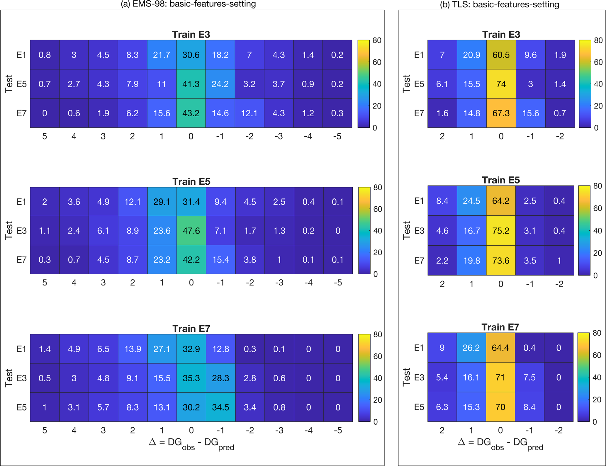
NHESS - Testing machine learning models for heuristic building damage assessment applied to the Italian Database of Observed Damage (DaDO)